

The Law of Equi-Marginal Utility is a fundamental concept in economics that helps explain how rational consumers allocate their limited resources among various goods and services to maximize their satisfaction or utility.
As we know that there is one defect in the law of diminishing marginal utility that it only explains the behavior the consumer as a regarding whole. Therefore, a particular consumer commodity law of equi-marginal at each time utility. It does be not developed explain which is an extension of the law of diminishing marginal utility.
This is used for maximizing total utility. The household maximizing its utility will allocate its income among commodities so that the utility of the last penny spent on each is equal. This law does not mean that a prudent consumer substitutes one item for the other in order to satisfy the same want e.g. tea and coffee.
It means that the consumer demands different items within his purchasing power and denies maximum utility from them. This is what every normal consumer desires.
Law of Equi-Marginal Utility Graph & Table
The Law of Equi-Marginal Utility is a fundamental concept in economics that helps explain how rational consumers allocate their limited resources among various goods and services to maximize their satisfaction or utility. Graphs and tables are often used to illustrate this concept and make it more tangible.
Law of Equi- Marginal Utility Graph
Imagine a consumer who has a fixed budget and is considering allocating it between two goods: A and B. The consumer seeks to maximize their total utility, which represents the satisfaction or benefit derived from consuming these goods. The graph will have the following components:
- X-axis: This represents the quantity of good A consumed.
- Y-axis: This represents the quantity of good B consumed.
Indifference Curve: An indifference curve is a curve that shows all the combinations of goods A and B that yield the consumer the same level of satisfaction or utility. These curves are typically downward-sloping, reflecting the Law of Diminishing Marginal Utility.
Budget Constraint Line: This line represents the consumer’s budget constraint. It shows all the combinations of goods A and B that the consumer can afford given their fixed budget and the prices of the goods.
Equilibrium Point: The point where the indifference curve is tangent to the budget constraint line represents the consumer’s equilibrium. At this point, the consumer has allocated their budget in a way that maximizes their utility, considering the marginal utility of both goods and their prices.
Law of Equi-Marginal Utility Table
A table can accompany the graphical representation to provide a more detailed view of how the consumer makes choices based on marginal utility. Here’s an example of such a table:
| Money ($) | Orange (M.U) | 7UP (M.U) |
|---|---|---|
| 1 | 5 | 20 |
| 2 | 10 | 15 |
| 3 | 15 | 10 |
| 4 | 20 | 05 |
| 5 | 25 | 00 |
Let us now explain the table. The consumer has $5 to spend and he wants to purchase these two items and derive maximum utility from them. Therefore, if he spends a certain amount of money on oranges. The rest he must spend on 7-Up
- If he spends $1 on oranges, he will benefit 25 utils and from the remaining $4 on 7-Up, he will benefit a total of 50 utils (20 + 15 + 10 + 5). Hence the total utility of this expenditure will be 75 utils.
- If he spends $2 on oranges, he will benefit 45 utils (25 + 20) and from the remaining $3 on 7-Up. he will benefit 45 utils (20 + 15 + 10). Ilea-ace total! a utility will be 90 utils.
- If he spends $3 on oranges, he will benefit 60 utils and from the remaining $2 on 7-Up he will benefit 35 utils (20 +15). Hence total utility will be 95 utils.
- If he spends $4 on oranges, he will benefit 70 utils and from the remaining Re. I on 7-Up he will benefit 20 utils. Hence, total utility will be 90 utils.
- If he spends $5 on oranges, he will benefit 75 utils and nothing from 7-Up! This is because he has spent all his money on oranges, which was not his intention, mainly because he wants to purchase two items and derive maximum utility from both.
Therefore, if the consumer? wants to benefit maximum satisfaction of both items and also wants to make full use of his purchasing power.
It is advisable for him to take the third case, i.e. $3 on oranges and $2 on 7-Up. He will get a total utility 95 utils… maximum satisfaction! (Which is more than in any other combination above).
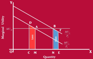
The following diagram shows rationality of the decision made by the consumer. In this case, his total utility will fall because marginal utilities of the goods are not equal.
This is evident from the gain and loss of utility shown in the diagram. We find that the gain of utility by spending an extra rupee on oranges is less than the loss of utility from 7-Up. Therefore, the difference between the two is the net loss in total utility.
Limitations of Law of Equi-Marginal Utility
We know that there are important assumptions of the law, but there are several limitations of the law, which should be discuss in detail. The main limitations of the law of Equi-Marginal utility are given below
-
Quantitative Measurement of Utility
Utility represents our feelings of satisfaction. The consumer only imagines the numerical value of the commodity in the form of utils.
See Also: Law Of Diminishing Marginal Utility | Assumptions & Limitations
It is not possible to actually quantify it, because it is only hypothetical. In other words, cardinal measurement of utility is not possible, hence, it is a limitation of the law.
-
Indivisibility of Certain Articles
we are able to get the marginal and total utility of small items because they are divisible such as apples or any other type of fruits, bottles drinks etc.
However, when it comes to big items such as fridge, television, cars etc, it is not possible to get their equi-marginal utility as the products are indivisible.
-
Time Period
When measuring the marginal and total utility of perishable goods such as” food, we are able to get a definite answer.
However, when we consider the case of durable goods this law does not hold. The reason is that the life time of these items is not the same, for example a pen and a watch.
Based on the fact that these two items are consumed continuously, the watch will have a longer life, hence this law does not hold.
-
Ignorance of Consumers
Generally, the consumers do not care very much for the price that they are paying for a certain item, e.g. at one shop the consumer purchases a pen for $20, but when he goes into another shop.
He finds that the similar pen is of $10. Hence, the consumer is not able to attain maximum satisfaction.
-
Carelessness of Consumers
In the case of usage of commodities under certain customs/traditional. a heavy price is paid for a negligible amount of utility obtained, e.g., for a wedding ceremony, a bride purchases a dress for $10,000, just for the sake of using it once.
See Also: Importance of Consumer Behavior
In this case it becomes difficult to equalize the marginal utility of different goods and also difficult to maximize total utility under the law of equi-marginal utility,
Importance of Law of Equi-marginal Utility
-
Guidance for Consumers
Any prudent consumer would naturally desire maximum total utility for the most minimum expenditure possible. In arranging his expenditure until he meets this point.
He will have to substitute a good with a greater utility, for one that possesses less utility, until the marginal utilities of the commodities purchased are equalized.
Thus, he will attain optimum use of these commodities, e.g. in our previous case of oranges and 7-Up.
The consumer purchased less of 7-Up because its marginal utility was greater than that of oranges $3 of oranges gave him a total utility of 60 utils and additional 30 utils for $2 of 7-UP’ hence his expenditure of $5 gave him total utility of 90 utils:
-
Guidance for Entrepreneurship
Marginal productivity theory has been derived from the law of Equi-marginal utility.
This theory enables a producer to maximize total production and profit combining the factors of production, i.e. land, labor, capital and entrepreneurship at the most possible minimum cost.
Produce equilibrium is also called least cost of factors of production “or” optimum combination of factor of production”
See Also: Methods of Economics | Methodology of Economics
However, the producer detects the marginal productivity of one of the factors is greater than the other.
For example, land’s marginal productivity is greater than that of capital’ marginal productivity, it will benefit him to substitute the land for the capital in order to get maximum profit.
-
Guidance for the Finance Minister
The finance minister has two duties, one to impose taxes, and the second is to take care of welfare expenditure.
In the case of imposing tax, he has to always have in mind that the community consists of two main classes or categories High Class and Low-Class people.
The former, being wealthier, naturally will be taxed more than the latter. But the question is” How much more “? and How much Less “?
Simple is to high class community feels on the payment of taxes is not as bad as how it is felt by the lower-class community.
Such as, if the High-class community that earns $100000/- annually has to pay $10000/- as tax each year.
The same rate cannot be imposed on lower class community with an equally a monthly income of $10000/.
Therefore, in order to equally distribute the burden of taxation on the whole society so that the marginal sacrifice of all tax-payers is equalized, the finance minister will refer to this law.
The money being spent has to be divided in such a way that the marginal social welfare of expenditure on different projects is equalized. In this way maximum social welfare will be attained.
See Also: What is Macro Economics | Merits and Demerits
-
Guidance for Fair Distribution of Wealth in the Society
In accordance with the producer’s equilibrium, marginal product of the four factors of production is to be equalized and the marginal product of each factor is also to be equal to its respective reward.
This would be the equal distribution of wealth or income in a country. Thus, with the attainment of the producer’s equilibrium fair distribution of wealth can be achieved in the whole society.
Assumptions of the Law of Equi-Marginal Utility
Law of Equi-Marginal Utility built upon a set of assumptions that form the basis for understanding consumer behavior and decision-making. Let’s discuss these assumptions one by one in detail.
1. Rational Consumer Behavior
At the core of the Law of Equi-Marginal Utility lies the assumption of rational consumer behavior. It assumes that consumers are rational individuals who aim to maximize their satisfaction (utility) given their limited resources, such as income. Rational consumers make choices that lead to the highest level of satisfaction, seeking to optimize their well-being.
2. Diminishing Marginal Utility
A fundamental assumption is the concept of diminishing marginal utility. It posits that as a consumer consumes more units of a particular good or service, the additional satisfaction (utility) derived from each additional unit decreases. In other words, the law assumes that consumers experience diminishing returns in terms of satisfaction as they consume more of a single item.
3. Fixed Income and Prices
The Law of Equi-Marginal Utility assumes that a consumer’s income and the prices of goods and services remain fixed during the analysis. This simplifies the analysis by isolating the impact of consumer choices on utility. In reality, income and prices can fluctuate, affecting consumer decision-making.
4. Independent Goods
It is assumed that the goods and services under consideration are independent of each other. This means that the consumption of one good does not directly affect the consumption of another. Consumers can make choices independently without constraints imposed by complementary or substitute goods.
5. Continuity and Transitivity
Continuity and transitivity are assumptions related to consumer preferences. Continuity assumes that consumers can make infinitesimal changes in their consumption, allowing for precise analysis of choices. Transitivity implies that if a consumer prefers option A to option B and option B to option C, they must also prefer option A to option C. These assumptions ensure consistency in consumer preferences.
6. Perfect Knowledge
The law assumes that consumers have perfect knowledge about the goods and services available in the market, including their prices and the satisfaction (utility) they derive from consuming them. Perfect knowledge enables consumers to make informed choices and optimize their utility.
7. Static Analysis
The Law of Equi-Marginal Utility is often applied in a static context, focusing on a single point in time. It does not consider dynamic factors such as changes in consumer preferences over time or the long-term effects of choices. Real-world consumer behavior may involve evolving tastes and preferences.
8. No Externalities
The law assumes that the consumption of goods and services does not create externalities or spillover effects on others. In reality, some consumption choices can have social, environmental, or health-related externalities that impact society at large.
The Law of Equi-Marginal Utility | Graph | Table | Limitations | Assumptions | Importance | PDF Free Download |
Conclusion
The Law of Equi-Marginal Utility serves as a valuable framework for understanding how rational consumers allocate their resources to maximize satisfaction. Its assumptions simplify the analysis of consumer behavior, but they may not always hold in complex, dynamic, and imperfectly informed real-world scenarios. Recognizing these assumptions allows economists to model and analyze consumer choices while acknowledging the inherent complexities of decision-making.