

An indifference curve is a graph that shows different combinations of two goods or services that provide an individual with an equal level of satisfaction or utility. Indifference curves are essential in understanding consumer preferences, especially in microeconomics. Different authors and economists have provided various definitions and insights into indifference curves. Here are a few definitions by different authors:
- Francis Y. Edgeworth defined indifference curve as a “locus of points showing all combinations of goods that give the consumer the same level of satisfaction.”
- Alfred Marshall described indifference curves as “lines that represent all the combinations of two goods between which a consumer is indifferent.”
- Paul Samuelson: says indifference curve is a geometric representation of all the combinations of two goods that yield the same level of satisfaction to a consumer.
An indifference curve is a contour line that slopes downward from left to right, showing equal levels of satisfaction on each of its points, with the given amount of income spent on different combinations.
As the indifference curve is always convex to the origin it shows that the Marginal Rate of Substitutions (MRS) gradually falls, to enable the consumer to move from one combination to another of two commodities or more. Key characteristics of indifference curve are as under:
- Equal Satisfaction: All points along the curve represent bundles of goods that yield an equal level of satisfaction or utility to the consumer. In other words, the consumer is indifferent between any two points on the same curve.
- Downward Sloping: Indifference curves typically slope downward from left to right. This means that as the quantity of one good increase, the quantity of the other good must decrease to maintain the same level of satisfaction.
- Convex Shape: Indifference curves are generally convex to the origin (bowed inward). This convexity reflects the principle of diminishing marginal rate of substitution, which means that consumers are willing to trade off less of one good for more of another but at a diminishing rate.
- Non-Intersecting: Indifference curves do not intersect with each other. If they did, it would imply that a consumer is indifferent between two different levels of satisfaction, which is not possible.
- Higher Curve, Higher Satisfaction: A higher indifference curve represents a higher level of satisfaction. Consumers aim to reach higher indifference curves whenever possible.
- Tangent to Budget Constraint: An optimal consumption point is where an indifference curve is tangent to the consumer’s budget constraint, representing the highest level of satisfaction attainable given the budget.
Properties of Indifference Curves
The properties of indifference curves are crucial for understanding consumer preferences and choices in microeconomics. These properties help economists analyze how consumers make decisions based on their preferences for various combinations of goods and services. Here are the key properties of indifference curves:
- Negatively Sloped: Indifference curves slope downward from left to right. This means that as a consumer increases the quantity of one good while keeping the consumption of the other good constant, the level of satisfaction (utility) remains the same. The negative slope reflects the concept of the diminishing marginal rate of substitution (MRS), where consumers are willing to give up less of one good to gain more of another.
- Convex to the Origin: Indifference curves are typically convex to the origin, which means they bend inward as they move away from the origin. This convexity indicates that consumers exhibit a diminishing marginal rate of substitution. In other words, consumers become less willing to trade one good for another as they move along the indifference curve.
- Cannot Intersect: Indifference curves for a single consumer cannot intersect with each other, If they did intersect, it would imply that the consumer is equally satisfied with two different combinations of goods, which contradicts the concept of rational consumer choice. A unique level of utility we see in each indifference curve.
- Higher Indifference Curve Represents Higher Utility: As we move away from the origin, toward the upper-right side of the graph, we encounter indifference curves that represent higher levels of utility. This indicates that consumers prefer higher utility (greater satisfaction) to lower utility.
- Indifference Maps: A collection of indifference curves for a single consumer is called an “indifference map.” These maps provide a comprehensive view of a consumer’s preferences for various combinations of goods. Higher indifference curves (farther from the origin) represent greater satisfaction.
- Diminishing Marginal Rate of Substitution: The marginal rate of substitution (MRS) decreases as indifference curve move from left to right. This reflects the decreasing willingness of consumers to trade one good for another while keeping their satisfaction constant.
- Transitivity: Transitivity is a property of preferences implied by indifference curves. If a consumer prefers bundle A to bundle B and bundle B to bundle C, then they must also prefer bundle A to bundle C. Indifference curves align with the principle of transitivity in consumer preferences.
- Completeness: Completeness implies that consumers can compare and rank all possible combinations of goods. For any two bundles of goods, consumers can indicate a preference for one over the other or express indifference.
- Monotonicity: Monotonicity means that consumers generally prefer more of each good to less. An increase in the quantity of at least one good, while holding the other constant, should lead to a higher level of satisfaction. Indifference curves align with this preference pattern.
These properties of indifference curves provide a foundation for understanding how consumers make choices in the face of scarcity. They allow economists to analyze consumer preferences, optimize choices, and make predictions about consumer behavior in various economic scenarios.
Indifference Curve Graph and Table
As we know that indifference curve is a fundamental concept in microeconomics used to illustrate consumer preferences and choices. They show various combinations of two goods or services that provide the same level of satisfaction or utility to a consumer.
Indifference Curve Graph
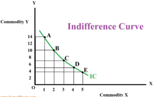
In the graph below, we’ll consider a hypothetical consumer, Alex, who is making choices between Commodity X and Commodity Y. The two axes represent the quantities of Commodity X (x-axis) and Commodity Y (y-axis). The indifference curve (IC) represents combinations of Commodity X and Commodity Y that provide the same level of satisfaction to Alex.
Indifference Curve Table
| Combination | Commodity X | Commodity Y | Total Utility |
|---|---|---|---|
| A | 1 | 10 | 50 |
| B | 2 | 7 | 50 |
| C | 3 | 5 | 50 |
| D | 4 | 4 | 50 |
In this table:
- Combination A represents zero units of Commodity X and four units of Commodity Y, yielding a total utility of 50.
- Combination B consists of one unit of Commodity X and five units of Commodity Y, providing the same total utility of 50.
- Combination C consists of two units of Commodity X and seven units of Commodity Y, also resulting in a total utility of 50.
- Combinations D and E similarly provide the same total utility of 50 by varying the quantities of Commodity X and Commodity Y.
Understanding the Indifference Curve:
- Downward Sloping Curve: As we move from Combination X to Combination Y along the indifference curve, the quantity of one good decreases while the quantity of the other increases. This is why indifference curves are downward-sloping.
- Equal Utility: Alex is indifferent between these combinations because they all provide the same level of satisfaction (total utility of 50). The curve connects all these combinations.
- Diminishing Marginal Rate of Substitution: The principle of diminishing marginal rate of substitution is evident. Alex is willing to give up fewer Y to gain an additional cup of X as we move to the right along the curve. The rate of substitution decreases as we go from Combination X to E.
- Convex Shape: The curve is convex to the origin, indicating that the trade-off between X and Y becomes less favorable as we move to the right. This reflects the diminishing marginal utility of each good.
The indifference curve illustrates the preferences of the consumer. To maximize utility, Alex would choose a combination that is on the highest possible indifference curve and still affordable, given their budget constraint.
This concept of indifference curves helps economists analyze consumer choices and understand how changes in prices and income impact consumption decisions.
Assumptions of Indifference Curve
The analysis of indifference curves in microeconomics is based on several fundamental assumptions that help us understand consumer preferences and choices. These assumptions are as follows:
- Transitivity: Consumers are assumed to be rational, meaning they have clear preferences and can make consistent choices. Transitivity assumes that if a consumer prefers bundle A to bundle B and bundle B to bundle C, then they must prefer bundle A to bundle C. In other words, preferences are logically consistent.
- Completeness: This assumption implies that consumers can compare and rank all possible bundles of goods. When faced with two different combinations of goods, consumers are capable of determining which one they prefer, even if it’s a matter of indifference.
- More Is Better: This assumption suggests that, in general, having more of a good is preferred to having less. In other words, goods are desirable, and consumers strive to increase their consumption of goods.
- Non-Satiation: This is often called the assumption of “wanting more.” It implies that consumers always prefer more of a good to less. In economic terms, there’s no point at which a consumer says they’ve had “enough” of a good. More is always better.
- Diminishing Marginal Rate of Substitution: This is a key assumption specifically related to indifference curves. It suggests that as a consumer moves along an indifference curve (keeping utility constant), they are willing to give up smaller and smaller amounts of one good to obtain more of the other good. In simpler terms, the trade-off between the two goods becomes less steep as you move along the curve.
- Convexity: The assumption of convexity is related to the diminishing marginal rate of substitution. It means that indifference curves are typically convex to the origin. This convexity implies that the consumer is willing to trade off goods at a diminishing rate. In other words, the consumer is less willing to give up one good for more of the other as they consume more.
These assumptions are fundamental to the concept of indifference curves and are used to build models that help economists analyze consumer choices, preferences, and behavior. They provide a theoretical framework for understanding how individuals make decisions about what to consume given their budget constraints and the prices of goods.
Limitations of Indifference Curve
While indifference curves are a valuable tool for analyzing consumer preferences and choices, they also come with limitations. Understanding these limitations is crucial for applying the model effectively. Here are some of the key limitations of indifference curve analysis:
- Cardinal Measurement: Indifference curve analysis is based on the cardinal utility approach, which assumes that utility can be measured in absolute units (utils). This concept has limitations because utility is a subjective measure, and there’s no universal standard for measuring it. Different individuals may assign different values to the same level of utility.
- Income and Wealth Effects: The model does not consider income and wealth effects. Changes in a consumer’s income or wealth can lead to shifts in their budget constraint and, consequently, changes in their preferences and consumption patterns. The indifference curve analysis assumes a fixed budget constraint.
- Inadequate Treatment of Necessities and Luxuries: The model treats all goods as substitutes or complements, regardless of whether they are necessities (e.g., basic food items) or luxuries (e.g., expensive vacations). In reality, consumers may have different preferences for necessities and luxuries, and the model doesn’t account for these distinctions.
- Limited Realism: Indifference curves are simplifications of real-world consumer behavior. They assume that consumers make choices based solely on utility and do not consider psychological or sociological factors that influence consumption decisions.
- Constant Marginal Rate of Substitution: While diminishing marginal rates of substitution are assumed along an indifference curve, this assumption doesn’t always hold true in practice. In some cases, consumers may face corner solutions where they only consume one of the two goods.
- Single Consumer Model: The model focuses on the behavior of a single consumer. In reality, many consumption decisions are made by households or families, and individual preferences may not always align with the choices made at the household level.
- Time Frame: The model assumes that preferences remain stable over time. However, consumer preferences may change due to factors like changing demographics, trends, or new information.
- Complexity of Preferences: Consumer preferences are often multifaceted and can involve various considerations beyond the consumption of goods, such as brand preferences, ethical concerns, and social influences. The model simplifies preferences into a two-dimensional space.
- Non-Convex Preferences: While the model assumes convex preferences (diminishing marginal rate of substitution), some consumers may exhibit non-convex preferences, particularly when dealing with discrete goods or imperfect substitutability.
Despite these limitations, indifference curve analysis remains a valuable tool for understanding consumer choices and rational decision-making within the framework of certain assumptions. Economists recognize its usefulness while also acknowledging its simplifications and constraints when applied to real-world scenarios.
Importance of Indifference Curve
The significance of indifference curves in economics lies in their role as a foundational tool for understanding and analyzing consumer preferences, choices, and behavior. Here are the key aspects of their significance:
-
Consumer Preferences Analysis:
Indifference curves provide a graphical representation of how consumers make choices between different combinations of goods and services. They help economists understand how consumers rank and evaluate various consumption bundles based on their preferences.
-
Optimal Consumer Choices:
By combining indifference curves with budget constraints, economists can determine the consumption bundle that maximizes a consumer’s utility, subject to their income limitations. This is critical for understanding how consumers allocate their resources among different goods and services.
-
Utility Maximization:
Indifference curves are central to the concept of utility maximization. Consumers aim to reach the highest possible level of satisfaction (utility) given their budget. This process is essential for both microeconomic analysis and consumer theory.
-
Consumer Surplus:
Indifference curves help in calculating consumer surplus, which is the difference between what consumers are willing to pay for a good and what they actually pay. This concept is crucial for assessing the welfare of consumers resulting from different market conditions.
-
Market Demand Analysis:
Indifference curve analysis allows for the aggregation of individual demand curves to derive market demand curves. This helps in understanding the overall demand for a product in a market.
-
Welfare Economics:
In welfare economics, indifference curves are used to assess changes in consumer welfare resulting from shifts in market prices or policy changes. This is particularly relevant for evaluating the impacts of economic policies and market interventions.
-
Labor-Leisure Tradeoff:
Indifference curves can be applied to analyze the labor-leisure tradeoff. It helps in understanding how individuals make choices between work and leisure time, which is essential for labor economics.
-
Investment and Saving Decisions:
Economists use indifference curve analysis to examine how individuals make decisions about saving and investing. It provides insights into the choices people make between current consumption and future income.
-
Comparative Statics:
Indifference curve analysis allows for comparing the effects of changes in prices, income, or preferences on consumer choices. This is vital for understanding how economic variables impact consumer behavior.
-
Teaching and Learning Tool:
Indifference curves are widely used in economics education to illustrate economic concepts and demonstrate how consumers make choices. They serve as a valuable pedagogical tool.
Indifference curves are indispensable for understanding consumer behavior and preferences, optimizing consumer choices, assessing welfare implications, and making important economic policy decisions. They are a fundamental component of microeconomic analysis and provide valuable insights into how individuals allocate their resources in a world of scarcity.
Indifference Curve | Graph | Table | Assumptions | Limitations | Importance | PDF Free Download |
Conclusion
Indifference curves are crucial for understanding consumer behavior, utility maximization, and the concept of marginal rate of substitution, which helps determine how much of one good a consumer is willing to give up to acquire one more unit of another good while maintaining the same level of satisfaction. This analysis is fundamental in microeconomics for studying consumer choices and market demand.