What is Aggregate Supply | Importance | Components | Curve | Examples | Limitations

Aggregate supply is a fundamental concept in macroeconomics that plays a pivotal role in understanding how an economy functions. It represents the total quantity of goods and services that producers are willing and able to supply at various price levels.

This concept is crucial in determining an economy’s performance, inflationary pressures, and long-term economic growth.

In this article, we will talk about aggregate supply, what it is, its components, the short-run and long-run aspects, the factors influencing it, and the real implications of aggregate supply.

See Also: What is Law of Supply

What is Aggregate Supply | Different Definitions

Aggregate supply or AS is a fundamental concept in economics that represents the total quantity of goods and services that all producers in an economy are willing and able to supply at various price levels over a specific time period. Here are different definitions of aggregate supply by various authors:

1. John Maynard Keynes defined aggregate supply as the total amount of goods and services that firms in an economy are willing and able to supply at a given overall price level in a given time period. He distinguished between short-run and long-run aggregate supply.
2. Milton Friedman emphasized the importance of money supply in determining aggregate supply. He argued that in the long run, changes in the money supply affect nominal variables, such as prices, but not real variables, like the quantity of goods produced.
3. Paul Samuelson defined aggregate supply as the total quantity of goods and services that firms in an economy are willing and able to supply at various price levels. He also introduced the concept of the aggregate supply curve, which illustrates the relationship between overall price levels and the quantity of output supplied.
4. Alfred Marshall says aggregate supply as the combined supply of all individual firms in an economy. He highlighted that changes in costs, such as wages and raw material prices, can influence aggregate supply.
5. Robert Lucas argued that aggregate supply is primarily determined by technology and economic incentives. He believed that government policies and changes in money supply have little effect on aggregate supply in the long run.

These definitions provide different perspectives on the concept of aggregate supply and highlight the role of factors such as production costs, technology, monetary policy, and the time horizon in shaping an economy’s aggregate supply.

Understanding these definitions is crucial for comprehending an economy’s behavior and its response to various economic shocks and policy changes.

The Aggregate Supply Curve

The Aggregate Supply (AS) curve is a critical concept in macroeconomics that illustrates the total quantity of goods and services that an economy is willing and able to produce at different price levels.

There are two main components of the Aggregate Supply curve: the Short-Run Aggregate Supply (SRAS) and the Long-Run Aggregate Supply (LRAS). Let’s delve into each component in detail:

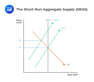
Short-Run Aggregate Supply Curve

The SRAS curve represents the total output that an economy can produce in the short run. It is positively sloped, indicating that, in the short run, as overall prices increase, the quantity of goods and services supplied also increases.

Several factors explain this upward slope:

1. Sticky Wages and Prices: In the short run, wages and many prices don’t adjust immediately to changes in demand. This stickiness means that when prices rise, businesses may produce more to take advantage of higher revenues, resulting in an upward-sloping SRAS curve.
2. Capacity Utilization: Firms may not be operating at full capacity in the short run. With increased demand due to price rises, they can increase output without incurring additional production costs.
3. Resource Price Adjustment Lag: It takes time for resource prices (like oil or labor) to adjust to changes in demand or supply. When prices rise, firms can produce more in the short run, given existing contracts and agreements.
4. Diminishing Returns: As output increases, firms may experience diminishing returns to labor and capital, making it less profitable to produce more as prices rise.

In essence, the SRAS curve illustrates the idea that an economy can expand its production in the short run in response to price increases.

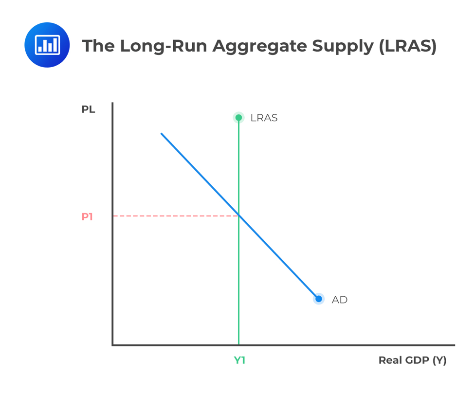
Long-Run Aggregate Supply Curve

The LRAS curve represents the total output an economy can produce when all factors of production, including capital and labor, are fully employed. It is vertical, indicating that, in the long run, changes in the overall price level do not affect the economy’s total output.

The LRAS curve is vertical because in the long run, factors that determine an economy’s productive capacity are flexible:

1. Full Employment: In the long run, all available labor and capital are fully utilized.
2. Flexible Wages and Prices: In contrast to the short run, wages and prices have fully adjusted to market conditions, making them more responsive to changes in demand.
3. Technological Progress: Technological advancements can increase an economy’s productive capacity. In the long run, these advancements are factored into production, resulting in a higher level of potential output.
4. Economic Growth: Over time, an economy can expand its productive capacity through investments in capital, human capital, and technology.
5. Resource Allocation: The long run allows for resources to shift toward their most productive uses. Firms can adapt to changing market conditions, and the economy operates at its maximum potential output.

The Aggregate Supply curve in economics is a representation of the economy’s ability to produce goods and services at different price levels. The short run (SRAS) shows a positive relationship between prices and production due to various factors’ short-term stickiness.

In contrast, the long run (LRAS) assumes full flexibility and responsiveness of prices and resources, resulting in a vertical curve. Understanding these concepts is crucial for analyzing economic fluctuations and the impacts of economic policies on an economy’s output.

Importance of Aggregate Supply

Aggregate Supply is a fundamental concept in macroeconomics with significant importance in understanding an economy’s functioning, its fluctuations, and the implications of various economic policies. Here’s an in-depth explanation of the importance of Aggregate Supply:

1. Understanding Economic Growth:

Aggregate Supply helps economists and policymakers gauge a nation’s potential economic growth. The Long-Run Aggregate Supply (LRAS) curve represents the maximum sustainable output level when all resources are fully utilized. Monitoring this curve allows us to assess an economy’s growth prospects and potential for increasing living standards.

2. Analyzing Inflation:

Aggregate Supply plays a vital role in assessing inflationary pressures. When the Short-Run Aggregate Supply (SRAS) curve is steep and the LRAS curve is not reached, the economy is likely operating below its potential. This situation can lead to inflation as firms respond to increased demand by raising prices. Conversely, if the economy operates along the LRAS curve, inflationary pressures are minimized.

3. Evaluating Economic Stagnation:

A flat SRAS curve implies that the economy’s resources are fully utilized, leaving little room for expansion. In such cases, fiscal or monetary policies may be needed to stimulate economic growth. Understanding Aggregate Supply helps identify economic stagnation and informs policy decisions to counter it.

4. Policy Decisions:

Policymakers often use the Aggregate Supply model to determine the appropriate actions during economic downturns. If the economy is operating below its potential (on the SRAS curve’s left side), expansionary policies, like tax cuts or increased government spending, can be employed to boost output. If the economy is operating beyond its potential (right side of the SRAS curve), contractionary policies, such as raising interest rates or reducing government spending, can help mitigate inflation.

5. Price Stability:

Analyzing Aggregate Supply is crucial for maintaining price stability. By examining the position of the SRAS curve in relation to the LRAS curve, economists can identify whether an economy is prone to inflation or deflation. Achieving a balance between Aggregate Supply and Aggregate Demand is essential for ensuring stable prices.

6. Labor Market Insights:

Understanding Aggregate Supply assists in assessing the labor market. A steep SRAS curve may indicate that there’s still a surplus of unemployed labor and underutilized capital. Conversely, a flat SRAS curve suggests a tight labor market where further increases in output might lead to higher labor costs and, subsequently, inflation.

7. Long-Term Planning:

For businesses, investors, and policymakers, Aggregate Supply is vital for long-term planning and decision-making. It provides insights into future production capabilities, potential growth opportunities, and whether resource constraints might limit future expansion.

8. Economic Resilience:

The Aggregate Supply model helps economists understand an economy’s ability to withstand shocks. A robust LRAS curve represents an economy that can quickly recover from adverse events, such as recessions or supply disruptions. The model aids in assessing an economy’s resilience and preparedness for such challenges.

Aggregate Supply is a critical concept in economics that facilitates the understanding of an economy’s potential output, inflationary pressures, and the need for economic policies. It plays a key role in macroeconomic analysis and policy formulation, helping stakeholders make informed decisions to achieve economic stability and growth.

The Components of Aggregate Supply

Aggregate supply, often abbreviated as AS, consists of two main components: the Short-Run Aggregate Supply (SRAS) and the Long-Run Aggregate Supply (LRAS). These components represent an economy’s production capability over different time horizons.

They help us understand the dynamics of how an economy responds to changes in factors such as prices, wages, and technology. Let’s break down these components for a better understanding.

Short-Run Aggregate Supply (SRAS)

Short-run aggregate supply (SRAS) refers to the total output that an economy is willing and able to produce over a relatively short period, typically up to a few years. It is a crucial element in analyzing an economy’s performance in the near term.

The SRAS curve shows the relationship between the price level (P) and the total quantity of goods and services supplied (Q) by producers. It generally exhibits a positive slope, indicating that as prices rise, producers are willing to supply more output. Conversely, when prices fall, they may reduce their production.

Factors Influencing SRAS

Several factors influence the position of the SRAS curves, including:

1. Input Costs: Fluctuations in the prices of key production inputs such as labor, raw materials, and energy can impact SRAS.
2. Technological Advances: Innovations that improve productivity can shift the SRAS curve to the right, increasing output.
3. Government Regulations: Changes in regulations can affect producers’ costs, which, in turn, influence SRAS.
4. Business Expectations: Producers’ expectations about future economic conditions can impact their willingness to invest in production.

Long-Run Aggregate Supply (LRAS)

Long-run aggregate supply (LRAS) represents the economy’s production potential over an extended period, typically several years to decades. It portrays the maximum sustainable level of output an economy can achieve when all resources are fully employed, and all markets are in equilibrium.

The LRAS curve is typically depicted as vertical, indicating that it is unaffected by changes in the price level. This suggests that in the long run, changes in the overall price level have no bearing on an economy’s production capacity. Instead, LRAS is determined by factors such as labor force size, technological progress, and the availability of physical and human capital.

Factors Influencing LRAS

The primary factors that influence the position of the LRAS curve include:

1. Population Growth: An expanding labor force can shift the LRAS curve to the right, leading to increased long-term production capacity.
2. Technological Advancements: Ongoing technological progress is a key driver of economic growth and the long-run supply of goods and services.
3. Investment in Human Capital: Policies that enhance education and skills development can boost LRAS.
4. Infrastructure Development: Improving an economy’s infrastructure can have a long-lasting impact on its productive capacity.

Macroeconomic Equilibrium

Achieving macroeconomic equilibrium is a critical goal in economic policymaking. It refers to the point at which the aggregate supply (AS) equals aggregate demand (AD) in an economy. When an economy reaches this equilibrium, it experiences stable price levels and a level of production that matches demand. Let’s explore how macroeconomic equilibrium is achieved and its implications for economic stability.

Achieving Equilibrium

Macroeconomic equilibrium occurs when the total quantity of goods and services supplied by producers (AS) is equal to the total quantity demanded by consumers, businesses, and the government (AD). The aggregate supply and aggregate demand curves intersect at this point, determining the equilibrium price level and the equilibrium level of output.

In this balanced state, prices are stable, and there is no upward or downward pressure on inflation. The economy is operating at its potential output, and the labor market is in a state of full employment. Achieving this equilibrium is a primary objective of macroeconomic policy.

Implications for Economic Stability

The macroeconomic equilibrium is associated with economic stability and balanced growth. When supply aggregate matches aggregate demand, the following implications are observed:

1. Price Stability: There are no inflationary or deflationary pressures. Prices remain relatively constant, contributing to a predictable business environment.
2. Full Employment: The economy is operating at its potential output, resulting in lower unemployment rates.
3. Balanced Growth: An economy at equilibrium experiences consistent and balanced growth, reducing the likelihood of economic downturns.

Now, let’s explore the factors that can cause shifts in aggregate supply, disrupting this equilibrium and influencing economic conditions.

Shifts in Aggregate Supply

Shifts in aggregate supply represent changes in the total quantity of goods and services that all producers in an economy are willing and able to supply at different price levels. These shifts can result from various factors and have important implications for an economy. Let’s explore the details of shifts in aggregate supply:

Factors Influencing Shifts in Aggregate Supply:

1. Changes in Resource Prices: When input prices, such as labor, raw materials, or energy, increase or decrease significantly, they can influence the cost of production. Higher resource prices lead to a decrease in aggregate supply (a leftward shift), while lower resource prices increase aggregate supply (a rightward shift).
2. Technological Advancements: Improvements in technology and increased productivity can positively impact aggregate supply. More efficient production methods, machinery, and automation can lead to higher output, resulting in an increase in aggregate supply (a rightward shift).
3. Taxes and Regulation: Government policies, such as changes in taxes or regulations, can affect business costs and productivity. Higher taxes or increased regulation might decrease aggregate supply (a leftward shift), while lower taxes or reduced regulation can boost aggregate supply (a rightward shift).
4. Macroeconomic Factors: Economic conditions, like inflation and exchange rates, can also influence aggregate supply. High inflation may lead to uncertainty and decreased supply, while stable prices can foster increased production.
5. Supply Shocks: Unexpected events, often related to natural disasters or geopolitical crises, can have significant impacts on aggregate supply. For instance, a natural disaster disrupting the supply of a critical resource can reduce aggregate supply (a leftward shift).

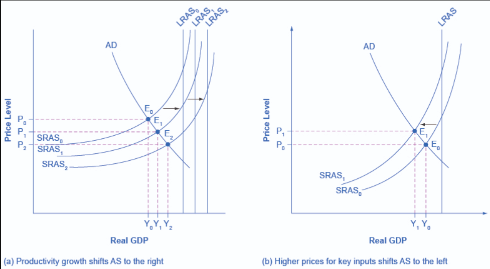
Shift in the Short-Run Aggregate Supply (SRAS) Curve:

In the short run, the SRAS curve can shift leftward or rightward due to these factors, leading to changes in the equilibrium price level and real GDP.

A leftward shift represents a decrease in aggregate supply, which may result in higher prices and reduced output. A rightward shift reflects an increase in aggregate supply, potentially leading to lower prices and increased output.

Implications for the Economy:

Shifts in aggregate supply have several economic implications. An increase in aggregate supply can lead to lower price levels, making goods and services more affordable for consumers. It can also support economic growth by allowing businesses to produce more.

A decrease in aggregate supply may lead to inflationary pressures if the economy operates near full capacity. It can also result in lower real GDP and potentially higher unemployment rates.

Shift in the Long-Run Aggregate Supply (LRAS):

The LRAS curve represents the economy’s production potential when all resources are fully employed. Changes in aggregate supply in the short run can impact the price level but not the long-run aggregate supply. The LRAS curve is considered vertical because, in the long run, changes in aggregate supply are reflected in price levels rather than output.

Shifts in aggregate supply can result from various factors, impacting an economy’s equilibrium price level and real GDP in the short run. Understanding these shifts is crucial for policymakers and economists to address economic challenges and maintain stability in the economy.

Examples of Aggregate Supply

Examples of aggregate supply help illustrate how real-world events and factors can influence the total quantity of goods and services that an economy produces. Here are some detailed examples:

1. Technological Advancements:

Technological progress often results in an increase in short-run aggregate supply (SRAS). For instance, the development of more efficient manufacturing processes or the use of automation in production can lead to higher output levels. An example could be the adoption of 3D printing technology in manufacturing, which allows for quicker and more cost-effective production, increasing aggregate supply.

2. Resource Price Changes:

Fluctuations in resource prices can significantly impact aggregate supply. A drop in the cost of energy, such as a decrease in oil prices, can lead to an increase in SRAS as it reduces production costs across various industries. On the other hand, a surge in energy prices due to geopolitical events may decrease SRAS.

3. Macroeconomic Policies:

Government policies can influence SRAS. Tax cuts and regulatory reforms can reduce business costs and promote economic growth, leading to an increase in aggregate supply. Conversely, an increase in corporate taxes and stricter regulations may hinder production and decrease aggregate supply.

4. Supply Shocks:

Supply shocks are sudden and unexpected events that can disrupt the supply of goods and services. Natural disasters like hurricanes, earthquakes, or floods can damage infrastructure, disrupt transportation, and lead to supply shortages, reducing aggregate supply. For example, Hurricane Katrina in 2005 disrupted oil production and refining in the Gulf of Mexico, causing a decrease in oil supply and driving up energy prices.

5. Labor Force Changes:

Changes in the size and skills of the labor force can impact aggregate supply. For instance, a surge in immigration can increase the labor force, potentially increasing aggregate supply. Conversely, if a large portion of the population retires, it may reduce the labor force and affect production.

6. Global Events and Trade:

International events can also affect aggregate supply. Trade tensions or conflicts can lead to tariffs or trade barriers, reducing the availability of imported goods. This can impact SRAS if businesses rely on foreign inputs. On the other hand, international trade agreements that open up new markets may lead to an increase in aggregate supply.

7. Global Pandemics:

Recent examples include the COVID-19 pandemic, which had a significant impact on global aggregate supply. Lockdowns, travel restrictions, and supply chain disruptions resulted in production slowdowns or stoppages across various industries. Conversely, the development of vaccines and the easing of restrictions contributed to a gradual recovery in aggregate supply.

8. Natural Resource Discoveries:

The discovery of new natural resources, such as oil reserves or minerals, can lead to an increase in aggregate supply. Countries with resource-rich environments can experience an economic boost as they extract and export these resources.

9. War and Conflict:

Armed conflicts can lead to disruptions in production and a decrease in aggregate supply. War can damage infrastructure, disrupt supply chains, and lead to the destruction of productive assets.

10. Government Investment:

Government investments in infrastructure, technology, and education can lead to increased human capital and better productivity. For example, a government-funded project to build efficient transportation systems can improve an economy’s SRAS.

These examples demonstrate how various factors and events can impact an economy’s ability to produce goods and services, emphasizing the dynamic nature of aggregate supply and its sensitivity to real-world changes and developments.

Limitations of Aggregate Supply

Aggregate Supply (AS) is a valuable concept in macroeconomics, but it also has its limitations. Understanding these limitations is crucial for a comprehensive analysis of an economy. Here are the key limitations of Aggregate Supply:

1. Assumes Homogeneous Output

The AS curve treats all goods and services as if they have uniform price behavior. In reality, different industries and products may exhibit varying responses to changes in demand, input prices, or productivity. This simplification can lead to imprecise conclusions.

2. Simplistic Price Expectations:

The AS model often assumes that firms and workers have perfect knowledge of future prices and wages. In practice, expectations are based on a wide range of factors, including past experiences, information, and psychological factors. These expectations may not always align with economic realities.

3. Ignores Imperfect Information:

The model assumes that firms, workers, and consumers have perfect information. In the real world, information is often imperfect, leading to uncertainty about future prices, wages, and market conditions. This can result in inefficient market responses.

4. Long-Run Equilibrium Assumptions:

The model relies on the concept of a long-run equilibrium where all input and output prices are flexible. However, in reality, some prices, like wages, may be sticky, leading to prolonged periods of economic imbalances.

5. Ignores Market Power:

The AS model typically assumes perfect competition. In reality, many markets are characterized by monopolistic or oligopolistic behavior. These firms have market power, which enables them to influence prices and output levels. Such market power can disrupt the predictions of the AS model.

6. Neglects Macroeconomic Variables:

The model primarily focuses on the supply side and does not incorporate other important macroeconomic variables like government policies, international trade, and aggregate demand. In the real world, these factors can significantly impact the economy.

7. Ignores Behavioral and Psychological Factors:

The model assumes that economic agents are entirely rational and make decisions solely based on maximizing utility or profit. In reality, behavioral and psychological factors often influence decisions, leading to outcomes that may not align with the model’s predictions.

8. Assumes Rational Expectations:

The AS model assumes that agents have rational expectations about the economy’s future state. In practice, expectations can be influenced by various cognitive biases, emotions, and information constraints, leading to deviations from rationality.

9. No Consideration of Income Distribution:

The model focuses on aggregate output and prices but doesn’t account for how the benefits of economic growth and price changes are distributed among different segments of society. Changes in income distribution can significantly impact the overall well-being of a nation.

10. Doesn’t Account for Market Failures:

The model assumes perfectly functioning markets, but real-world markets can suffer from various imperfections and failures, such as externalities, public goods, and information asymmetry. These market failures can disrupt the AS-AD equilibrium.

11. Static Analysis:

The AS model often provides a static view of an economy, assuming that all factors instantly adjust to changes. In reality, adjustments can take time, leading to periods of economic instability.

12. Disregards Political Factors:

The model doesn’t consider political factors, such as government stability, policy changes, or geopolitical events, which can have a substantial impact on an economy’s performance.

Despite these limitations, the Aggregate Supply model remains a valuable tool for analyzing an economy’s production capabilities and potential growth. However, it should be used in conjunction with other models and real-world data to provide a more comprehensive and accurate understanding of economic conditions and policies.

Conclusion

Aggregate supply is a critical concept in macroeconomics that helps us comprehend an economy’s production capabilities and how it interacts with other macroeconomic variables.

By dissecting the components of aggregate supply, such as SRAS and LRAS, and exploring their influencing factors, we gain a more profound understanding of how an economy functions in the short run and long run. Achieving macroeconomic equilibrium is a key goal in economic policymaking, as it brings stability and balanced growth.

However, shifts in aggregate supply, whether from positive or negative supply shocks, can disrupt this equilibrium, impacting an economy’s performance.

Understanding the real-world implications of aggregate supply analysis through historical events and economic policies provides valuable insights for policymakers and economists. In practice, aggregate supply is a dynamic force that shapes an economy’s trajectory, and a comprehensive grasp of this concept is indispensable for effective economic decision-making.

See Also: What is Aggregate Demand | Importance | Components | Curve | Limitations